Forecasting Ocean Plastic Around the Globe: A Deep Dive into Modeling the Garbage Patches

Before reading this article, you could think that discussing the creation of a global ocean plastic forecast, without even looking at any results, is already pretty shocking. Global models are usually used to study phenomena that have existed for billions of years, such as weather, climate evolution, or continental drift. So how could we, as a species, let the plastic pollution issue become big enough that we have to write about a global forecast for our own trash?

In 1965 the first piece of oceanic plastic was found in a plankton recording device in the ocean. More than half a century later, plastic pollution built up so much that you can find microplastics in your table salt. Recently, researchers have even estimated that every week you ingest the equivalent in microplastics of a credit card.

So, plastic is now practically everywhere.

At The Ocean Cleanup, we believe that to solve a problem one must thoroughly understand it first. If we are to clean this mess up, we need to learn more and ask questions like: how does it travel in the ocean, and where does it accumulate? This is why understanding the dynamics of ocean plastics and their impact around the globe is critical to us. And as always with such problems, it involves many different phenomena at various scales.

The Ocean Cleanup has several teams working on modeling different parts of the problem: in the ocean, in rivers, at small scales around the cleanup systems, near coasts, etc. To forecast ocean plastics distribution at the largest scale (the Earth), we use a so-called dispersion model. Below is a typical output of such a program in a simple case.

A simple dispersion model

Because this is a crucial element to our technology development and cleanup approach, we wanted to introduce you to our global plastic dispersion model by providing you with a basic explanation of the science behind the calculations. The results we produce may seem alarming, but they are quite insightful for the work of The Ocean Cleanup and the general public as well. And if you have some programming experience, you could learn enough to create your own model at home.

MODELING PLASTICS IN THE OCEAN: PRINCIPLES OF DISPERSION MODELING

The plastic dispersion models we use are Lagrangian models. Simply put, it means that our data consists of virtual particles, which are defined by their coordinates in time and their release date and location. What we do with them is also pretty straightforward: starting at their release date, we let them drift away in the ocean by using data about the currents, winds, and other phenomena at stake.

By doing this, one must realize that a particle trajectory over time is not a correct representation of what happens in real life. There are too many uncertainties, and, by nature, this process is chaotic. One slight change in release position and date can make the particle have very different trajectories. As in many other fields, dispersion modeling gets statistically accurate when increasing the number of particles.

The Ocean Cleanup global models use millions of particles or, in some cases, tens of millions. It’s at these massive scales that concentration zones appear plainly. There are five of these so-called oceanic garbage patches, and they are where most of the floating plastic ends its course, and where it will continue drifting for decades. The biggest one, in the North Pacific, is called the Great Pacific Garbage Patch (GPGP).

With this model, we observe that it takes approximately a decade for the majority of our initial virtual plastic particles to make their way to these concentration zones. Once this time has passed, we can assume that our data is ready to harvest in the form of concentration maps, which show the patches’ geography.

DRIVING PHENOMENA AND PLASTIC SOURCES

We are now ready to delve into the core of the dispersion model: the advection scheme . It revolves around a central differential equation that integrates all phenomena at stake to give an estimate of a particle velocity, or the plastic’s speed through water. Basically, our methods calculate the particle’s velocity at a given time with a formula and use it to estimate where the particle will be a few minutes later. We repeat this process over a long period of time to get a series of positions, i.e., a trajectory of where the plastic goes.

The advection equation currently in use at The Ocean Cleanup is similar to the following:

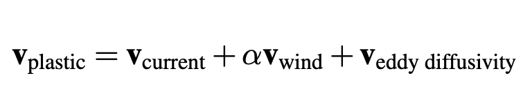
The advection equation: the addition of three terms. The role of α will not be explained in this article.

What this equation means is that each time we need to compute the speed of the plastic particle, we compute it as the sum of the speeds of three phenomena. Below is a simple example of what it looks like when we add wind and currents velocities.

Adding the current and wind speeds to get the plastic speed

This process is repeated each time we need to compute a particle speed.

You might then ask how we know the currents and wind speeds every time we need them.
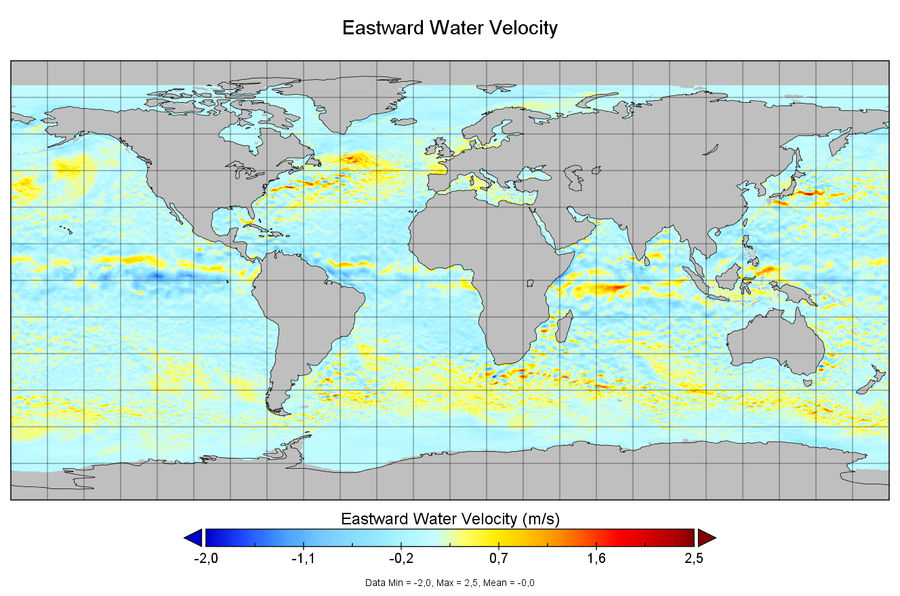
We calculate them through a process called interpolating. Essentially, we have immense datasets containing currents and winds at specific places and times, and we choose to use the value closest to the plastic particle. This process is illustrated below, repeated twice.

Finding the closest current speed and using it to move the plastic

After using winds and currents, we need to take into account eddy diffusivity. This concept represents small-scale phenomena we are unable to model because they happen at scales that are too small for our computers to simulate. Practically, modeling it simply consists of moving the particle randomly around its position with a tiny displacement, a mathematical process called a random walk.

Our complete process, repeated over time, is illustrated below. The red arrow represents the random walk: every time a new one is generated in a random direction, with a random size.

Complete process with three particles.

As this process has to be repeated over years, the datasets containing wind and speeds all around the globe can take up a lot of space. For instance, the LLC4320 global circulation model uses no less than 5 petabytes of data to be stored. At The Ocean Cleanup, we often use HYCOM data for currents (illustrated below), and GFS for the wind; and our datasets require at least 1.5 terabytes to be stored.

There is one last thing missing: the generation of the particles. If the advection scheme is the engine, the particles represent the fuel of the model. You need a lot of it to start seeing helpful stuff, and the results of a simulation can widely vary depending on where and when particles are generated.

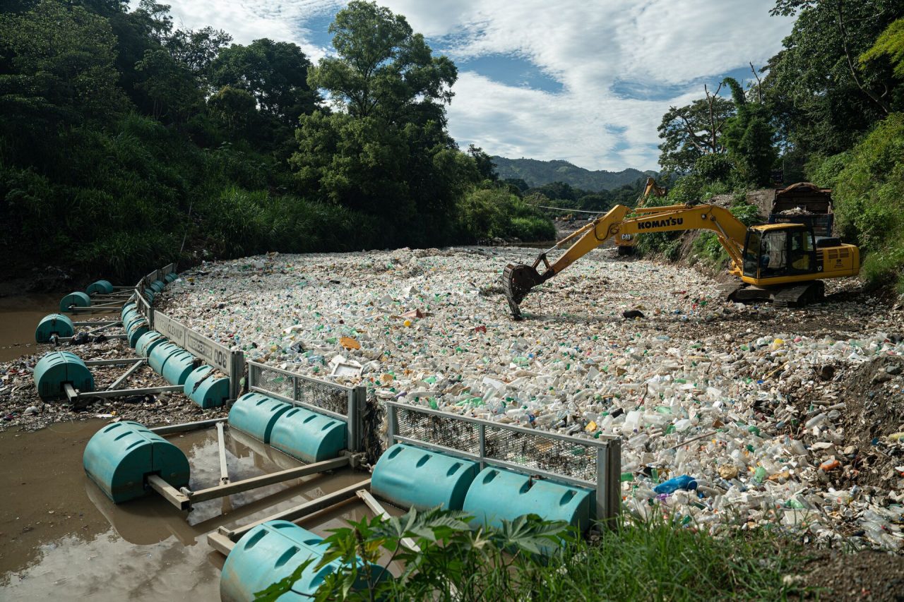
We have several models to generate particles around the world. For example, two that we often use are called “river sources” and “fishing sources”. For the former, plastic particles are generated at the estuary of rivers depending on the estimated throughput of plastic. Fishing source models generate particles directly in the ocean and represent plastic released by fishing boats, including ghost nets that amount to a significant part of the plastic mass in the patches. The generation rate depends on the activity in fishing zones around the world.

Below is an example of a simulation with river sources, focused on the Philippines, with particles generated in large streams from specific places on the coast. These are the estuaries of rivers known to be carrying plastic pollution.

Creation of particles in the Philippines with a river source model

RESULTS OF GLOBAL DISPERSION

The first finding of this kind of model is how ubiquitous plastic pollution is. Even with a few million particles (which is way less than the trillions of real drifting plastics), we can see it in every corner of the globe.

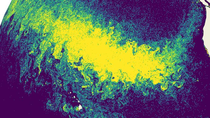
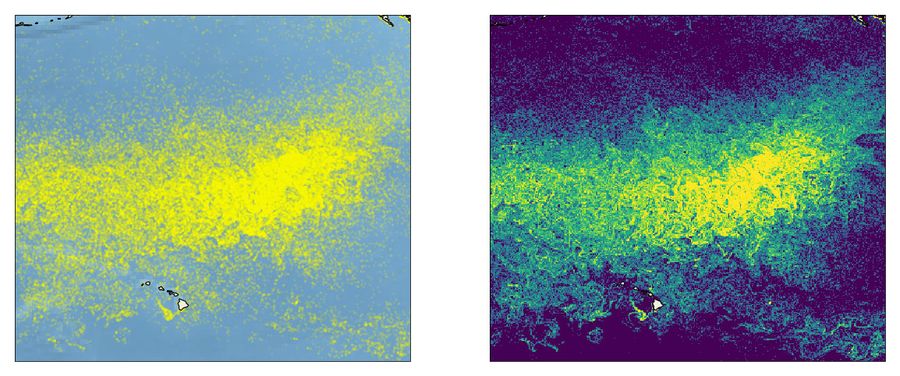
Zooming out of the GPGP

Now focusing on the concentration zones, the picture above illustrates the dynamics leading to the formation of the Great Pacific Garbage Patch (GPGP), one of the five main oceanic garbage patches. The GPGP is the largest patch and has been extensively explored during the past decade; observations recorded in the patch have been shown to match the prediction of dispersion models.

As with every planet-scale model, this one is fascinating, but it also illustrates a frightening truth: pollution is building up quickly. Luckily, it provides valuable and necessary insights that help us to define and develop the optimal technologies to clean it up.

The other four garbage patches (top left: North Atlantic, bottom left: South Atlantic, top right: Indian Ocean, bottom right: South Pacific). While less dense than the GPGP, they are similar in size

Knowing where our trash accumulates allows us to make efforts to remove it before it harms the environment more than it already has. At The Ocean Cleanup, we chose to create our offshore cleanup systems to capture and concentrate plastic debris in the garbage patches and our Interceptor technology, to also prevent plastic from reaching the oceans in the first place. And around the world, numerous organizations are roaming the oceans to retrieve ghost nets and other drifting trash and collecting trash from coastlines. It is a huge undertaking, but one we can all agree is necessary to preserve the health and life of this essential part of our planet.

Finally, for those with programming experience (or interest), there are great online tools to contribute to the efforts in improving plastic dispersion models. It is currently a hot scientific domain, one that is being developed by many teams worldwide, and their tools are mostly open. In fact, if you want to run your own simulations, there are open-source, easy-to-use modules for you to start exploring and contributing, such as OceanParcels or OpenDrift.

And if you want to roll up your sleeves and help us out by joining the team, check out our Careers page for the list of current vacancies.